Table manipulation

Pandas, short for Python Data Analysis Library, is a modern, powerful and feature rich library that is designed for doing data analysis in Python. Here, we will cover some basic Pandas that will allow you to store results in table format, do some basic table operations, visualization, and to read and write tables to files. You will find more information online in the Pandas Tutorials and in chapter 3 of the Python Data Science Handbook [VanderPlas, 2016].

import numpy as np
import pandas as pd
pd.__version__

'2.3.3'

DataFrame

The main pandas data structure is a table format called DataFrame. A DataFrame contains an Index and it contains columns. Columns are one-dimensional arrays of a single type called Series. A DataFrame can be created from a:

• single Series object

• list of dicts

• dictionary of Series objects

• two-dimensional NumPy array

• NumPy structured array

mySeries = pd.Series(['London', 'Paris', 'Berlin'], name='City', dtype='string')
cities = pd.DataFrame({"City": mySeries, "Population": [8.8, 2.2, 3.6]})
cities

	City	Population
0	London	8.8
1	Paris	2.2
2	Berlin	3.6

DataFrames have the following attributes: dtypes, shape, index, columns, values, empty.

cities.columns

Index(['City', 'Population'], dtype='object')

cities.dtypes

City          string[python]
Population           float64
dtype: object

cities.shape

(3, 2)

cities.values

array([['London', 8.8],
       ['Paris', 2.2],
       ['Berlin', 3.6]], dtype=object)

Reading and writing

The pandas library can read a variety of data formats using pandas.read_*(), including CSV, JSON, HTML, HDF5, Excel, SQL, SPSS, SAS, etc.:

fname = '../../data/airquality.csv'
airq = pd.read_csv(fname, index_col=0)
airq.head()

	Ozone	Solar	Wind	Temp	Month	Day
ID
101	41.0	190.0	7.4	67	5	1
102	36.0	118.0	8.0	72	5	2
103	12.0	149.0	12.6	74	5	3
104	18.0	313.0	11.5	62	5	4
105	NaN	NaN	14.3	56	5	5

The DataFrame object contains to_*() methods to write it to a file or database, e.g. airq.to_csv(out_filename).

Inspect DataFrame

DataFrames have several methods that are useful for inspection: head(), tail(), and describe()

airq.describe()

	Ozone	Solar	Wind	Temp	Month	Day
count	116.000000	146.000000	153.000000	153.000000	153.000000	153.000000
mean	42.129310	185.931507	9.957516	77.882353	6.993464	15.803922
std	32.987885	90.058422	3.523001	9.465270	1.416522	8.864520
min	1.000000	7.000000	1.700000	56.000000	5.000000	1.000000
25%	18.000000	115.750000	7.400000	72.000000	6.000000	8.000000
50%	31.500000	205.000000	9.700000	79.000000	7.000000	16.000000
75%	63.250000	258.750000	11.500000	85.000000	8.000000	23.000000
max	168.000000	334.000000	20.700000	97.000000	9.000000	31.000000

Select columns

airq.Ozone

ID
101    41.0
102    36.0
103    12.0
104    18.0
105     NaN
       ... 
249    30.0
250     NaN
251    14.0
252    18.0
253    20.0
Name: Ozone, Length: 153, dtype: float64

…or using a name or a list of names.

airq["Ozone"].head()

ID
101    41.0
102    36.0
103    12.0
104    18.0
105     NaN
Name: Ozone, dtype: float64

airq[["Ozone", "Solar"]].head()

	Ozone	Solar
ID
101	41.0	190.0
102	36.0	118.0
103	12.0	149.0
104	18.0	313.0
105	NaN	NaN

Asign new column

airq["logOzone"]  = np.log(airq.Ozone)
airq.head()

	Ozone	Solar	Wind	Temp	Month	Day	logOzone
ID
101	41.0	190.0	7.4	67	5	1	3.713572
102	36.0	118.0	8.0	72	5	2	3.583519
103	12.0	149.0	12.6	74	5	3	2.484907
104	18.0	313.0	11.5	62	5	4	2.890372
105	NaN	NaN	14.3	56	5	5	NaN

Select rows

Slicing

Slicing in pandas lets you select a continuous range of rows using start and end indices. It follows Python’s slicing rules, meaning it uses integer positions and the end index is exclusive. This provides a quick way to grab a block of consecutive rows. However, this syntax can be confusing because df[...] is also used for column selection, so airq[2:4] may look like it’s selecting columns when it’s actually slicing rows. Using .iloc is clearer, since it explicitly signals positional row access and avoids this ambiguity.

airq[2:4]

	Ozone	Solar	Wind	Temp	Month	Day	logOzone
ID
103	12.0	149.0	12.6	74	5	3	2.484907
104	18.0	313.0	11.5	62	5	4	2.890372

Boolean indexing

Boolean indexing in pandas selects rows based on a condition that evaluates to True or False for each row. It allows filtering data according to one or more logical expressions and supports combining conditions with logical operators (&, |, and ~). This method is flexible and one of the most commonly used ways to subset DataFrames.

Note: Under the hood, boolean indexing works by creating a mask of True and False values that determines which rows are selected.

airq[(airq.Ozone > 15) & (airq.Ozone < 18)]

	Ozone	Solar	Wind	Temp	Month	Day	logOzone
ID
112	16.0	256.0	9.7	69	5	12	2.772589
182	16.0	7.0	6.9	74	7	21	2.772589
195	16.0	77.0	7.4	82	8	3	2.772589
243	16.0	201.0	8.0	82	9	20	2.772589

Query

The query() method in pandas provides a way to filter rows using a string expression, making complex conditions more readable and concise. It can handle multiple conditions and logical operators, and even allows referencing variables from the environment using @.

month = 5
airq.query("Month == @month and Day < 5")

	Ozone	Solar	Wind	Temp	Month	Day	logOzone
ID
101	41.0	190.0	7.4	67	5	1	3.713572
102	36.0	118.0	8.0	72	5	2	3.583519
103	12.0	149.0	12.6	74	5	3	2.484907
104	18.0	313.0	11.5	62	5	4	2.890372

Select rows and columns

Unlike the previous selection methods, .loc and .iloc can select both rows and columns at the same time. .loc is label-based, meaning you select rows and columns using their index labels or column names. .iloc is position-based, meaning you select rows and columns by integer positions.

Using the iloc indexer, we can index the underlying array as if it is a simple NumPy array (using the implicit Python-style index), but the DataFrame index and column labels are maintained in the result:

airq.iloc[1:3, 2:4]

	Wind	Temp
ID
102	8.0	72
103	12.6	74

Similarly, using the loc indexer we can index the underlying data in an array-like style but using the explicit row index and column indices:

airq.loc[100:102, ["Wind", "Temp"]]

	Wind	Temp
ID
101	7.4	67
102	8.0	72

Chained indexing

To extract rows and columns, we may chain the commands pulling the columns and then the rows or vice versa (order does not matter). However, we should avoid chained indexing as it can lead to unpredictable results and warnings. Instead, we should use .loc or .iloc for clarity and reliability.

The expression below is an example of chained indexing. First, airq[["Ozone", "Solar"]] selects the two columns, creating a new temporary DataFrame (See View vs Copy ). Then, [airq.Ozone > 130] tries to filter rows on that temporary DataFrame using a condition from the original DataFrame. The problem with this approach is that it can lead to unexpected behavior or warnings, because pandas is unsure whether the row filtering is applied to a view of the original DataFrame or a copy. This can cause issues if you later try to modify the filtered DataFrame.

airq["Ozone"][airq.Ozone > 130] = 130

/var/folders/d6/_vs0dtkd76d27wvhhz0_nn7h0000gn/T/ipykernel_44437/4132742754.py:1: SettingWithCopyWarning: 
A value is trying to be set on a copy of a slice from a DataFrame

See the caveats in the documentation: https://pandas.pydata.org/pandas-docs/stable/user_guide/indexing.html#returning-a-view-versus-a-copy
  airq["Ozone"][airq.Ozone > 130] = 130

A safer alternative is to use .loc, which avoids chaining:

airq.loc[airq.Ozone > 130, "Ozone"] = 130

Methods

You can do masking and other useful things directly via methods of Series and DataFrames., e.g.

• airq.Ozone.between(15, 18)

• airq.Month.isin([5, 8])

• airq.Month.astype(“string”)

airq.isna().sum()

Ozone       37
Solar        7
Wind         0
Temp         0
Month        0
Day          0
logOzone    37
dtype: int64

Simple aggregation functions include mean(), median(), min(), max(), and std().

airq['Ozone'].mean()

np.float64(41.758620689655174)

Grouping

Sometimes we want to apply aggregation functions for individual factors separately.

airq.groupby('Month')

<pandas.core.groupby.generic.DataFrameGroupBy object at 0x119914980>

Sometimes we want to apply aggregation functions for individual factors separately.

airq.groupby('Month').mean()

	Ozone	Solar	Wind	Temp	Day	logOzone
Month
5	23.615385	181.296296	11.622581	65.548387	16.0	2.812076
6	29.444444	190.166667	10.266667	79.100000	15.5	3.236673
7	58.923077	216.483871	8.941935	83.903226	16.0	3.883834
8	58.500000	171.857143	8.793548	83.967742	16.0	3.845345
9	31.448276	167.433333	10.180000	76.900000	15.5	3.218795

Groupby comes with additional aggregation methods that provide more flexibility: aggregate(), filter(), transform(), and apply().

airq.groupby('Month').aggregate(["min", "max", "mean"])

	Ozone			Solar			Wind			Temp			Day			logOzone
	min	max	mean	min	max	mean	min	max	mean	min	max	mean	min	max	mean	min	max	mean
Month
5	1.0	115.0	23.615385	8.0	334.0	181.296296	5.7	20.1	11.622581	56	81	65.548387	1	31	16.0	0.000000	4.744932	2.812076
6	12.0	71.0	29.444444	31.0	332.0	190.166667	1.7	20.7	10.266667	65	93	79.100000	1	30	15.5	2.484907	4.262680	3.236673
7	7.0	130.0	58.923077	7.0	314.0	216.483871	4.1	14.9	8.941935	73	92	83.903226	1	31	16.0	1.945910	4.905275	3.883834
8	9.0	130.0	58.500000	24.0	273.0	171.857143	2.3	15.5	8.793548	72	97	83.967742	1	31	16.0	2.197225	5.123964	3.845345
9	7.0	96.0	31.448276	14.0	259.0	167.433333	2.8	16.6	10.180000	63	93	76.900000	1	30	15.5	1.945910	4.564348	3.218795

Append

Append rows

The stack two data.frames together by row, use the concat() function. Note append() will be depreciated in future versions of pandas.

pd.concat([airq.head(2), airq.tail(2)])

	Ozone	Solar	Wind	Temp	Month	Day	logOzone
ID
101	41.0	190.0	7.4	67	5	1	3.713572
102	36.0	118.0	8.0	72	5	2	3.583519
252	18.0	131.0	8.0	76	9	29	2.890372
253	20.0	223.0	11.5	68	9	30	2.995732

Append columns

The concat() function can also be used to stack columns of DataFrames together. The row index is preserved with an outer join by default.

pd.concat([airq.head(2), airq.tail(2)], axis=1)

	Ozone	Solar	Wind	Temp	Month	Day	logOzone	Ozone	Solar	Wind	Temp	Month	Day	logOzone
ID
101	41.0	190.0	7.4	67.0	5.0	1.0	3.713572	NaN	NaN	NaN	NaN	NaN	NaN	NaN
102	36.0	118.0	8.0	72.0	5.0	2.0	3.583519	NaN	NaN	NaN	NaN	NaN	NaN	NaN
252	NaN	NaN	NaN	NaN	NaN	NaN	NaN	18.0	131.0	8.0	76.0	9.0	29.0	2.890372
253	NaN	NaN	NaN	NaN	NaN	NaN	NaN	20.0	223.0	11.5	68.0	9.0	30.0	2.995732

To ignore row indices when stacking columns, you need to clear them prior to calling pd.concat().

df1 = airq.head(2).copy().reset_index(drop=True)
df2 = airq.tail(2).copy().reset_index(drop=True)
pd.concat([df1, df2], axis=1)

	Ozone	Solar	Wind	Temp	Month	Day	logOzone	Ozone	Solar	Wind	Temp	Month	Day	logOzone
0	41.0	190.0	7.4	67	5	1	3.713572	18.0	131.0	8.0	76	9	29	2.890372
1	36.0	118.0	8.0	72	5	2	3.583519	20.0	223.0	11.5	68	9	30	2.995732

Merge

Pandas implements several ways of combining datasets via the pd.merge() function and the join()methods of Series and DataFrames.

The pd.merge() function implements one-to-one, many-to-one, and many-to-many joins.

The pd.merge() function joins based on column names and not the Index. The column names can be explicitly defined via the keywords on, left_on, and right_on.

View vs Copy

When you create a new DataFrame by slicing an existing one, pandas often returns a view, not an independent copy. As a result, any modifications you make to that sliced DataFrame can unexpectedly alter the original data. To avoid accidental changes, explicitly create a copy when needed.

airq_view = airq.query("Month == 5 and Day < 5")
airq_view["Ozone"] = 0
airq.query("Month == 5 and Day < 5")

/var/folders/d6/_vs0dtkd76d27wvhhz0_nn7h0000gn/T/ipykernel_44437/3954834801.py:2: SettingWithCopyWarning: 
A value is trying to be set on a copy of a slice from a DataFrame.
Try using .loc[row_indexer,col_indexer] = value instead

See the caveats in the documentation: https://pandas.pydata.org/pandas-docs/stable/user_guide/indexing.html#returning-a-view-versus-a-copy
  airq_view["Ozone"] = 0

	Ozone	Solar	Wind	Temp	Month	Day	logOzone
ID
101	41.0	190.0	7.4	67	5	1	3.713572
102	36.0	118.0	8.0	72	5	2	3.583519
103	12.0	149.0	12.6	74	5	3	2.484907
104	18.0	313.0	11.5	62	5	4	2.890372

To avoid accidental changes, explicitly create a copy when needed.

airq_copy = airq.query("Month == 5 and Day < 5").copy()
airq_copy["Ozone"] = 0
airq_copy.query("Month == 5 and Day < 5")

	Ozone	Solar	Wind	Temp	Month	Day	logOzone
ID
101	0	190.0	7.4	67	5	1	3.713572
102	0	118.0	8.0	72	5	2	3.583519
103	0	149.0	12.6	74	5	3	2.484907
104	0	313.0	11.5	62	5	4	2.890372

Visualization

matplotlib

%matplotlib inline
import matplotlib.pyplot as plt
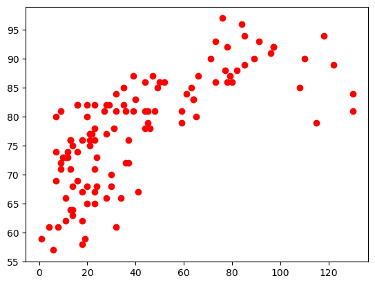
plt.plot(airq.Ozone, airq.Temp, 'or')
plt.show()

Pandas

Pandas provides visualization tools built on top of matplotlib. Hence, you still need to import matplotlib’s pyplot. You can read more in the pandas reference guide here. There are two ways to use pandas for plotting:

• via plot() methods for Series and DataFrames.

• via the plotting module pandas.plotting.

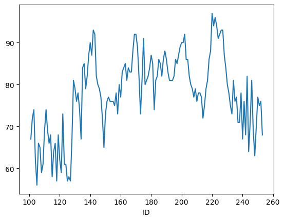
By default plot() shows a line graph using the row indices a x-axis and the columns as data lines:

airq.Temp.plot()
plt.show()

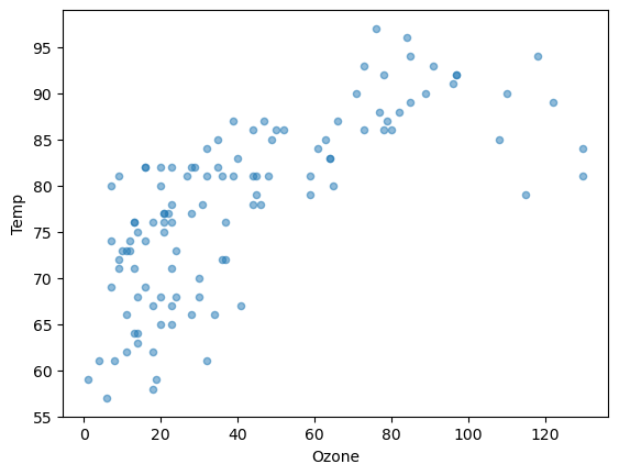
You can create other plots using the methods DataFrame.plot.kind or provide the kind keyword argument to the plot() method:

airq.plot.scatter(x="Ozone", y="Temp", alpha=0.5)
plt.show()